Adding Plots
In this section, we’ll add a plot to the t-test analysis we’ve been
developing in this series. A plot is another item to appear in the
results, so we’ll add another entry into our ttest.r.yaml
file:
---
name:  ttest
title: Independent Samples T-Test
jrs:   '1.1'

items:
    - name:  ttest
      title: Independent Samples T-Test
      type: Table
      rows:  1
      columns:
        - name: var
          title: ''
          type: text
        - name: t
          type: number
        - name: df
          type: integer
        - name: p
          type: number
          format: zto,pvalue

    - name: plot
      title: Descriptives Plot
      type: Image
      width:  400
      height: 300
      renderFun: .plot
Same as before, we define an item with a name,
title and a type; in this case the type is
Image. Additionally, we define renderFun which
is the name of the function responsible for rendering the image.
Whatever we specify as the render function, we must add as a private
member function to ttestClass in
ttest.b.R:
#' @export
ttestClass <- R6::R6Class(
    "ttestClass",
    inherit = ttestBase,
    private = list(
        .run = function() {
            formula <- paste(self$options$dep, '~', self$options$group)
            formula <- as.formula(formula)

            results <- t.test(formula, self$data)

            table <- self$results$ttest
            table$setRow(rowNo=1, values=list(
                var=self$options$dep,
                t=results$statistic,
                df=results$parameter,
                p=results$p.value
            ))
        },
        .plot=function(image, ...) {  # <-- the plot function

        })
)
Adding ggplot2
We’re going to use ggplot2 for plotting, so make sure
you have that installed. To use ggplot2 in this package/module, we need
to add some entries into the DESCRIPTION and NAMESPACE files. We add
ggplot2 to the imports line in the DESCRIPTION, so it reads:
Imports: jmvcore, R6, ggplot2and we’ll add the following line into NAMESPACE:
import(ggplot2)These entries are standard for using R code from other packages in a package. More information is available in Writing R Extensions.
Now we have ggplot2 ready, we can proceed with using it in our analysis.
Implementing Plots
In jamovi modules, plotting occurs in two stages; first the data for the plot is prepared, then the plot is rendered. The two stages mean that if the image is resized, or the user requests a different file format, only the rendering needs to be performed again — the data preparation needs only to occur once.
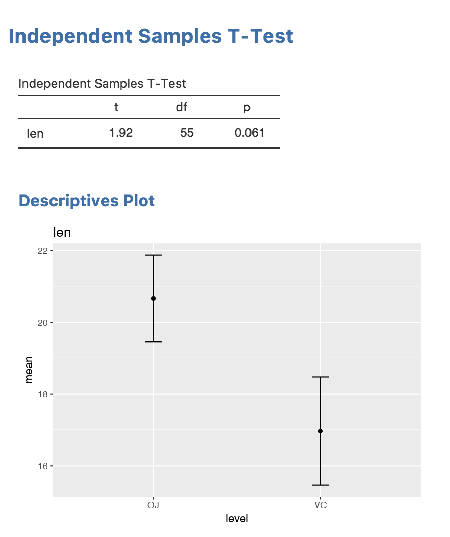
For the t-test, we’re going to plot a mean for each of the groups,
and the standard errors. In ggplot2, we’re required to
assemble these ‘plot points’ into a data frame, which we will do as
follows:
    means  <- aggregate(formula, self$data, mean)[,2]
    ses    <- aggregate(formula, self$data, function(x) sd(x)/sqrt(length(x)))[,2]
    sel    <- means - ses  # standard error lower bound
    seu    <- means + ses  # standard error upper bound
    levels <- base::levels(self$data[[self$options$group]])
    plotData <- data.frame(level=levels, mean=means, sel=sel, seu=seu)
## level mean sel seu
## 1 OJ 20.66333 19.45733 21.86934
## 2 VC 16.96333 15.45417 18.47250This plot data we assign to the image using the
setState() function:
Next, we’ll add the plotting code into the .plot()
function we created:
.plot=function(image, ...) {
plotData <- image$state
plot <- ggplot(plotData, aes(x=level, y=mean)) +
geom_errorbar(aes(ymin=sel, ymax=seu, width=.1)) +
geom_point(aes(x=level, y=mean)) +
labs(title=self$options$dep)
print(plot)
TRUE
}The plot function accepts an argument image, which
corresponds to the image object we called setState() on. We
can retrieve the state object from this image with
image$state, which we can see is being assigned to
plotData.
Following this are a number of calls to ggplot2
functions. A full discussion of how to use ggplot2 is well and
truly beyond the scope of this document, but there are many
excellent resources available online.
Next we explicitly print the ggplot object. When using ggplot
interactively in an R session, calling ggplot() leads to
the creation of the plot, however, when calling ggplot from inside a
function, it is necessary to explicitly call print().
The final statement is TRUE which is the return value.
Don’t forget this! Returning true notifies the rendering system that you
have plotted something. If you don’t return true, your plot will not
appear. There are situations where the user may not have specified
enough information for plotting, in which case the function should
return FALSE.
So this is our final ttest.b.R file:
#' @export
ttestClass <- R6::R6Class(
"ttestClass",
inherit = ttestBase,
private = list(
.run = function() {
formula <- paste(self$options$dep, '~', self$options$group)
formula <- as.formula(formula)
results <- t.test(formula, self$data)
table <- self$results$ttest
table$setRow(rowNo=1, values=list(
var=self$options$dep,
t=results$statistic,
df=results$parameter,
p=results$p.value
))
means <- aggregate(formula, self$data, mean)[,2]
ses <- aggregate(formula, self$data, function(x) sd(x)/sqrt(length(x)))[,2]
sel <- means - ses # standard error lower bound
seu <- means + ses # standard error upper bound
levels <- base::levels(self$data[[self$options$group]])
plotData <- data.frame(level=levels, mean=means, sel=sel, seu=seu)
    image <- self$results$plot
    image$setState(plotData)
},
    .plot=function(image, ...) {
        plotData <- image$state
        plot <- ggplot(plotData, aes(x=level, y=mean)) +
            geom_errorbar(aes(ymin=sel, ymax=seu, width=.1)) +
            geom_point(aes(x=level, y=mean)) +
            labs(title=self$options$dep)
        print(plot)
        TRUE
})
)And these are our final results, including the plot:
Next: Distributing Modules