Adding Plots

In this section, we’ll add a visual representation of our data. jamovi makes it easy to integrate ggplot2 to create beautiful plots.

1. Define the Image in YAML

Plots are items in your results, so we need to add an Image entry to jamovi/ttest.r.yaml.

# ... (existing ttest table)
    - name: plot
      title: Descriptives Plot
      type: Image
      width:  400
      height: 300
      renderFun: .plot

width & height: These set the initial dimensions of the plot in pixels. Because jamovi plots are vector graphics, the user can stretch and resize them later. These values simply define the default aspect ratio.
renderFun: .plot: This critically links your results definition to your R code. It tells jamovi exactly which function to call to draw this image. You can name this whatever you like (e.g., .renderMyPlot), as long as it perfectly matches the function name you’ll soon write in your R file.

2. Configure Dependencies

To use ggplot2, your module must declare it as a dependency in two files located in your project’s root directory:

DESCRIPTION: Add ggplot2 to the Imports: field. This tells R that your module requires this package to be installed.
```
Imports: jmvcore, R6, ggplot2
```
NAMESPACE: Add an import statement for ggplot2:
```
import(ggplot2)
```
Unlike the previous tutorial where we explicitly had to type stats::t.test(), adding this import statement loads all of ggplot2’s functions directly into your module’s memory. This means you can type clean code like ggplot() or geom_point() without having to attach the clunky ggplot2:: prefix to every single command.

3. The Plotting Model: State vs. Render

jamovi uses a two-stage system: Calculate data in .run(), draw it in .plot().

By saving data to the state, jamovi can redraw the plot instantly if the user resizes the window or changes a theme, without needing to re-run the entire analysis. This separation of concerns is key to a responsive UI.

Tip

Performance Tip: Summarizing your data in .run() before passing it to the plot state is a best practice. It keeps the state object small and ensures the .plot() function remains fast. See Image State Performance for more details.

4. Implementation in R

Open R/ttest.b.R and update your class definition.

ttestClass <- R6::R6Class("ttestClass",
    inherit = ttestBase,
    private = list(
        .run = function() {
            # 1. Input Check: Stop quietly if inputs are missing
            if (length(self$options$dep) == 0 || length(self$options$group) == 0) {
                return()
            }

            # -- 2. Existing Analysis & Table Logic --
            formula <- jmvcore::constructFormula(self$options$dep, self$options$group)
            formula <- as.formula(formula)

            results <- stats::t.test(formula, self$data, var.equal=self$options$varEq)

            table <- self$results$ttest
            table$setRow(rowNo=1, values=list(
                var = self$options$dep,
                t   = results$statistic,
                df  = results$parameter,
                p   = results$p.value
            ))

            # -- 3. NEW: Prepare Plot Data (State) --
            # Calculate means and standard errors for our plot
            means <- aggregate(formula, self$data, mean)[, 2]
            ses   <- aggregate(formula, self$data, function(x) sd(x) / sqrt(length(x)))[, 2]
            
            sel <- means - ses
            seu <- means + ses
            levels <- base::levels(self$data[[self$options$group]])

            plotData <- data.frame(
                level = levels,
                mean  = means,
                sel   = sel,
                seu   = seu
            )

            # Save the data to the image state
            image <- self$results$plot
            image$setState(plotData)
        },

        .plot = function(image, ...) {
            # 'image' is the R6 object representing the Image element
            # '...' allows for future arguments from the rendering system

            plotData <- image$state

            if (is.null(plotData))
                return(FALSE)

            p <- ggplot(plotData, aes(x = level, y = mean)) +
                geom_errorbar(aes(ymin = sel, ymax = seu), width = 0.1) +
                geom_point()

            # Return the ggplot2 object directly
            return(p)
        }
    )
)

Note

The Dot Prefix: Why did we name our function .plot instead of just plot? In jamovi, the dot prefix indicates that a method is private to your R6 class. You’ll notice that both .run and .plot sit inside the private = list(...) block. This keeps your public API clean while allowing the jamovi framework to safely call these methods internally.

Why return the plot object?

return(p) (Returning the Object): Unlike in an interactive R session where plots appear automatically, jamovi’s rendering system expects your .plot function to return the ggplot2 object (or a base R plot). jamovi then handles the printing to the appropriate graphics device.
return(TRUE) (Self-Printing Packages): Some R packages produce plots by calling print() or a similar function internally — the plot is sent directly to the active graphics device as a side effect. In this case, there is no object to return. Instead, call your plotting function (which prints the plot itself), then return TRUE to signal to jamovi that the plot was successfully rendered.
Success/Failure: If you return the plot object or TRUE, jamovi assumes success and renders it. If you return FALSE (or NULL), jamovi will assume the plot is empty or not yet ready and won’t display anything.

5. Test your Plot

Run jmvtools::install() in your R console. Open jamovi, select your analysis, and drag some variables into the slots. You should see your plot appear!

And the result will look like this:

final plot

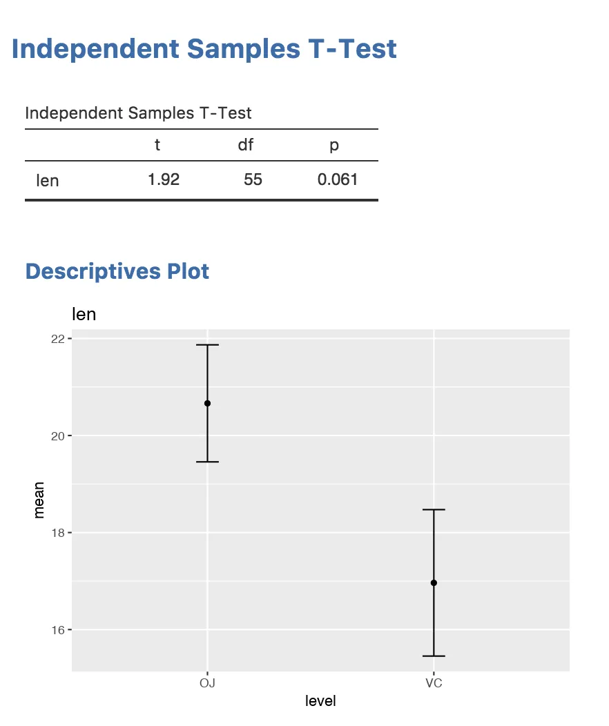
Next Step: Wrap up your first analysis and explore where to go next in the Getting Started Summary.